Comparison of two independent proportions#

To better understand how meta-analysis works, let’s examine a real-world example. We’ll focus on a section of the meta-analysis conducted by Eyding and colleagues, which investigated the effectiveness, measured as response rate, of reboxetine for treating severe depression [@eyding_reboxetine_2010]. This portion of their analysis includes seven studies, each providing an odds ratio (OR) and its corresponding 95% confidence interval. As we discussed in chapter @sec-comparing-proportions, an odds ratio serves as a measure of association. Specifically, in this context, an OR exceeding 1.0 indicates that reboxetine was more effective than the placebo, while an OR below 1.0 suggests it was less effective.

In this section, we will delve into the meta-analysis of counted data, focusing on methods used for comparing two independent proportions. We’ll explore how to implement this analysis using the statsmodels’ meta_analysis module in Python. Statsmodels provides a suite of tools that facilitate meta-analysis, offering functions for:

• Calculating effect sizes for comparing two independent proportions via effectsize_2proportions. This includes risk difference, (log) risk ratio, (log) odds-ratio, or arcsine square root transformation, along with their standard errors.

• Computing fixed and random effects estimates for the overall mean or effect via the combine_effects function, which also provides the ability to generate informative forest plots.

• Estimating the random effect variance, tau-squared, which is essential for random-effects models.

import io
import pandas as pd

raw_data_eyding = """
study,count_t,nobs_t,count_c,nobs_c
014,70,126,43,128
015,65,110,58,111
046,144,252,136,247
047,120,238,108,239
050,60,144,63,143
045,38,88,39,86
049,42,106,35,104
"""

data_eyding = pd.read_csv(
    io.StringIO(raw_data_eyding),
    converters={'study': lambda x: str(x)},
    index_col='study'
    )

print(data_eyding)

       count_t  nobs_t  count_c  nobs_c
study                                  
014         70     126       43     128
015         65     110       58     111
046        144     252      136     247
047        120     238      108     239
050         60     144       63     143
045         38      88       39      86
049         42     106       35     104

import numpy as np
from statsmodels.stats.meta_analysis import (
    effectsize_2proportions,
    combine_effects,
)

# Extract data for effect size calculation
count_t = data_eyding['count_t'].values
nobs_t  = data_eyding['nobs_t'].values
count_c = data_eyding['count_c'].values
nobs_c  = data_eyding['nobs_c'].values

# Calculate effect sizes (log odds ratios) and variances
eff_eyding, var_eyding = effectsize_2proportions(
    count1=count_t,
    nobs1=nobs_t,
    count2=count_c,
    nobs2=nobs_c,
    statistic="odds-ratio",  # We could also look at risk difference p1 - p2
)

print("Study list:\t", data_eyding.index.values)
print("Log odds ratios\t:", eff_eyding.round(2))
print("Log variance:\t", var_eyding.round(3))
print("Odds ratios\t:", np.exp(eff_eyding).round(2))
print("Variance:\t", np.exp(var_eyding).round(3))

Study list:	 ['014' '015' '046' '047' '050' '045' '049']
Log odds ratios	: [ 0.9   0.28  0.08  0.21 -0.1  -0.09  0.26]
Log variance:	 [0.067 0.074 0.033 0.034 0.057 0.093 0.082]
Odds ratios	: [2.47 1.32 1.09 1.23 0.91 0.92 1.29]
Variance:	 [1.069 1.077 1.033 1.034 1.059 1.098 1.086]

study_014 = data_eyding.loc[data_eyding.index == '014']
a, n1, c, n2 = study_014.iloc[0]

b, d = n1 - a, n2 - c
p1, p2 = a / n1, c / n2

log_or_014 = np.log(p1 / (1 - p1) / (p2 / (1 - p2)))
log_var_014 = (1 / a + 1 / b + 1 / c + 1 / d)

print("Effect size and variance for study '014':")
print(f"Log(OR) = {log_or_014:.2f} \
with Log(s²) = {log_var_014:.3f}")
print(f"OR = {np.exp(log_or_014):.2f} \
with s² = {np.exp(log_var_014):.3f}")

Effect size and variance for study '014':
Log(OR) = 0.90 with Log(s²) = 0.067
OR = 2.47 with s² = 1.069

# Perform meta-analysis (random-effects using chi2/DL method)
res_eyding = combine_effects(
    effect=eff_eyding,
    variance=var_eyding,
    method_re="chi2",  # One-step chi2/DerSimonian-Laird estimate for RE variance τ²
    use_t=False,
    row_names=data_eyding.index
)

# Print key information
print("Random effects (RE) method:", res_eyding.method_re)

# Print formatted summary results
print("\nMeta-analysis summary (log):\n", res_eyding.summary_frame())

Random effects (RE) method: chi2

Meta-analysis summary (log):
                         eff    sd_eff    ci_low    ci_upp      w_fe      w_re
014                0.904595  0.259159  0.396652  1.412537  0.115202  0.130693
015                0.277574  0.271507 -0.254571  0.809718  0.104962  0.123201
046                0.084557  0.180460 -0.269137  0.438252  0.237593  0.192509
047                0.209873  0.183578 -0.149932  0.569679  0.229590  0.189568
050               -0.097580  0.238630 -0.565287  0.370127  0.135876  0.144388
045               -0.087851  0.305341 -0.686309  0.510607  0.082989  0.105232
049                0.257545  0.287226 -0.305407  0.820497  0.093788  0.114410
fixed effect       0.205226  0.087962  0.032823  0.377629  1.000000       NaN
random effect      0.214617  0.118666 -0.017964  0.447198       NaN  1.000000
fixed effect wls   0.205226  0.115618 -0.021381  0.431833  1.000000       NaN
random effect wls  0.214617  0.122392 -0.025268  0.454501       NaN  1.000000

# Extract relevant summary statistics and exponentiate for odds ratios
res_eyding_or = np.exp(res_eyding.summary_frame().loc[
    :'random effect',  # We remove WLS
    ['eff', 'sd_eff', 'ci_low', 'ci_upp']
]).round(2)

print("Meta-analysis summary (ORs):\n", res_eyding_or)

Meta-analysis summary (ORs):
                 eff  sd_eff  ci_low  ci_upp
014            2.47    1.30    1.49    4.11
015            1.32    1.31    0.78    2.25
046            1.09    1.20    0.76    1.55
047            1.23    1.20    0.86    1.77
050            0.91    1.27    0.57    1.45
045            0.92    1.36    0.50    1.67
049            1.29    1.33    0.74    2.27
fixed effect   1.23    1.09    1.03    1.46
random effect  1.24    1.13    0.98    1.56

from scipy.stats import norm

# Defining critical z value for α=0.05 (z_crit ≈ 1.96)
z_crit = norm.ppf(q=(1 - 0.05/2))

ci_lo_log = log_or_014 - z_crit * np.sqrt(log_var_014)
ci_hi_log = log_or_014 + z_crit * np.sqrt(log_var_014)

ci_lo_or = np.exp(ci_lo_log)
ci_hi_or = np.exp(ci_hi_log)

print("Confidence intervals for study '014':")
print(f"95% CI of Log(OR) extends from {ci_lo_log:.4f} to {ci_hi_log:.4f}")
print(f"95% CI of OR extends from {ci_lo_or:.2f} to {ci_hi_or:.2f}")

Confidence intervals for study '014':
95% CI of Log(OR) extends from 0.3967 to 1.4125
95% CI of OR extends from 1.49 to 4.11

Forest plot#

To visualize the meta-analysis results, we construct a forest plot, also known as a blobbogram (@fig-forest), which graphically summarizes the findings from all included studies. We utilize the plot_forest method from the statsmodels meta-analysis output, leveraging the combined effect sizes we calculated previously.

#| label: fig-forest
#| fig-cap: "Forest plot of the reboxetine study (response rate), using a log scale for the odds ratio"

import matplotlib.pyplot as plt
from matplotlib.ticker import ScalarFormatter

fig = res_eyding.plot_forest(
    use_exp=True, # to show OR instead of logOR
)
fig.set_figwidth(3.5)
fig.set_figheight(3)

plt.axvline(x=1, ls='--', color='blue')
plt.xscale('log')

# By default, a logarithmic scale uses a LogFormatter
plt.gca().xaxis.set_major_formatter(ScalarFormatter())
plt.xticks([.33, .5, 1, 2, 3, 5])

plt.title('Forest plot -- Eyding study')
plt.xlabel('Odds ratio (95% CI)');

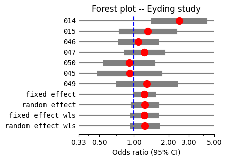
A forest plot uses horizontal lines to represent individual studies. Along each line, a square denotes the study’s effect size, and a line extending from the square represents the confidence interval. The position of markers indicates effect direction and magnitude, while confidence interval width reflects estimate uncertainty, and visual inspection can reveal heterogeneity across studies. Ideally, the square’s size would be proportional to the study’s weight in the meta-analysis, reflecting factors like sample size or precision, where larger squares imply greater influence. Currently, statsmodels doesn’t offer this feature, so in @fig-forest, a red dot of the same size is used to represent the effect size for all studies.

A vertical line, typically set at the value representing no effect (e.g., an odds ratio of 1), serves as a visual reference point. If a study’s confidence interval crosses this line, it suggests that the effect observed in that study is not statistically significant. Finally, a diamond shape at the bottom of the plot represents the pooled effect estimate, with its width indicating the confidence interval for the combined result.

Looking at the individual studies, six out of the seven have 95% confidence intervals for the odds ratio that include 1.0. This means we cannot confidently conclude that the drug is more effective than the placebo in those studies. However, one study shows a 95% CI that does not include 1.0, suggesting a statistically significant benefit in that particular study.

A key strength of meta-analysis lies in its ability to provide a more precise estimate of the overall effect by synthesizing evidence from multiple studies, even when individual studies exhibit heterogeneous findings. The confidence interval of the pooled effect is paramount for interpretation. If it includes the value representing “no effect,” such as 1.0 for odds ratios, we cannot confidently assert the presence of a genuine effect. Therefore, while statistical significance is important, clinical significance should also be considered, which involves evaluating the magnitude of the effect size.

Fixed-effects (Woolf method)#

When conducting a fixed-effects meta-analysis for comparing proportions, we often utilize the inverse-variance method, also known as the Woolf method. This approach widely used in meta-analyses, relies on a fundamental principle: assigning weights to studies based on the inverse of their variance.

# Fixed-effect weights (inverse variance)
fe_weights_eyding = res_eyding.weights_fe
print("\nFixed-effect weights (inverse variance):\n", fe_weights_eyding.round(3))

# Fixed-effect weights (normalized)
normalized_fe_weights_eyding = fe_weights_eyding / fe_weights_eyding.sum()
print("Normalized fixed-effect weights:\n", normalized_fe_weights_eyding.round(3))

Fixed-effect weights (inverse variance):
 [14.889 13.566 30.707 29.673 17.561 10.726 12.121]
Normalized fixed-effect weights:
 [0.115 0.105 0.238 0.23  0.136 0.083 0.094]

# Calculate combined effect size (fixed-effect)
E_eyding_fe = (eff_eyding * fe_weights_eyding).sum() / fe_weights_eyding.sum()

# Note that we can extract the effect size and weights as follows:
#E_eyding_fe = res_eyding.mean_effect_fe
#eff_eyding = res_eyding.effect
#fe_weights_eyding = res_eyding.weights_fe

# Calculate variance and standard error (fixed-effect)
var_eyding_fe = 1 / np.sum(fe_weights_eyding)
SE_eyding_fe = var_eyding_fe**0.5

# Calculate confidence interval (fixed-effect)

# If t-distribution is preferred, with k the number of studies
#from scipy.stats import t as t_dist
#t_crit_eyding = t_dist(df=res_eyding.df).ppf((1+.95)/2)
ci_lo_E_eyding_fe = E_eyding_fe - z_crit * SE_eyding_fe
ci_up_E_eyding_fe = E_eyding_fe + z_crit * SE_eyding_fe

print(f"Combined effect size (FE) = {E_eyding_fe:.3f}")
print(f"  with SE = {SE_eyding_fe:.4f}")
print(f"  and the 95% CI ranging from {ci_lo_E_eyding_fe:.4f} \
to {ci_up_E_eyding_fe:.4f}")
print(f"The 95% CI of the total OR (FE) of {np.exp(E_eyding_fe):.2f} \
extends from {np.exp(ci_lo_E_eyding_fe):.2f} to {np.exp(ci_up_E_eyding_fe):.2f}")

Combined effect size (FE) = 0.205
  with SE = 0.0880
  and the 95% CI ranging from 0.0328 to 0.3776
The 95% CI of the total OR (FE) of 1.23 extends from 1.03 to 1.46

Mantel-Hanszel odds-ratio#

Having thoroughly examined the inverse-variance weighted fixed-effects model, we now turn to another fixed-effects approach: the Mantel-Haenszel odds-ratio method, abbreviated MH. This technique, while still operating under the assumption of a common true effect across studies, utilizes contingency tables, discussed in @sec-comparing-proportions, to calculate a pooled odds ratio, particularly useful when dealing with binary outcomes.

In contrast to the inverse-variance method, which relies on continuous effect sizes and their variances, Mantel-Haenszel directly uses the counts within each study’s contingency table. While not typically a direct feature of standard meta-analysis functions within statsmodels, we can compute the Mantel-Haenszel odds-ratio using tools designed for stratified analysis, as demonstrated in another statsmodels tutorial. This necessitates transforming our data into a 2 x 2 x k table, specifically containing event and non-event counts, not event counts and total observations.

# Extract data into NumPy arrays
t = data_eyding['count_t'].values  # treatment
nt = data_eyding['nobs_t'].values  # total treatment
c = data_eyding['count_c'].values  # control
nc = data_eyding['nobs_c'].values  # total control

# Construct the 2 x 2 x k contingency table, containing
# event and non-event counts, in treatment and control
counts = np.column_stack([t, nt - t, c, nc - c])
ctables = counts.T.reshape(2, 2, -1)

# Print the first study contingency table for verification
print(f"Contingency table for study {data_eyding.index[0]}:")
print(ctables[:, :, 0])

Contingency table for study 014:
[[70 56]
 [43 85]]

We can apply the Mantel-Haenszel method using the StratifiedTable class to calculate the pooled log odds ratio and perform relevant statistical tests. In statsmodels, the Mantel-Haenszel confidence interval is calculated using the Robins, Breslow, and Greenland variance formula, or Sato’s method when necessary.

import statsmodels.stats.api as smstats

# Create a StratifiedTable object from the contingency table
# The contingency table is cast to float64 to ensure compatibility
st = smstats.StratifiedTable(ctables.astype(np.float64))

# Calculate and store the pooled log odds ratio
logodds_pooled = st.logodds_pooled

# Calculate and store the standard error of the pooled log odds ratio
logodds_pooled_se = st.logodds_pooled_se

# Calculate and store the confidence interval of the pooled log odds ratio
logodds_pooled_ci = st.logodds_pooled_confint()

# Print the results with formatted output
print(f"Pooled LogOR (MH) = {logodds_pooled:.4f}")
print(f"  with SE = {logodds_pooled_se:.4f}")
print(f"  and 95% CI of {np.round(logodds_pooled_ci, 4)}")

print(f"The 95% CI of the pooled OR (MH) of {np.exp(logodds_pooled):.2f} \
extends from {np.exp(logodds_pooled_ci[0]):.2f} to {np.exp(logodds_pooled_ci[1]):.2f}")

Pooled LogOR (MH) = 0.2067
  with SE = 0.0875
  and 95% CI of [0.0352 0.3782]
The 95% CI of the pooled OR (MH) of 1.23 extends from 1.04 to 1.46

While both methods, i.e., Woolf (inverse variance) and Mantel-Haenszel, estimate the pooled odds ratio under a fixed-effects assumption, their results are not entirely consistent. Among these, the Mantel-Haenszel method is generally considered the most robust, particularly in studies with small event counts [@lee_comparison_2016].

A chi-square test assesses if the pooled odds ratio differs from one.

# Perform a test of the null hypothesis that the pooled odds ratio is 1 (log odds = 0)
print("MH Test null OR:")
print(st.test_null_odds())

MH Test null OR:
pvalue      0.018042566133150473
statistic   5.5920114367536735

Beyond the Mantel-Haenszel method, Peto’s method can also be used for fixed-effects meta-analysis. However, Mantel-Haenszel is particularly advantageous in trials with sparse event data. The results of the Mantel-Haenszel test and calculations are summarized below.

print(st.summary())

                   Estimate   LCB    UCB 
-----------------------------------------
Pooled odds           1.230   1.036 1.460
Pooled log odds       0.207   0.035 0.378
Pooled risk ratio     1.112              
                                         
                 Statistic P-value 
-----------------------------------
Test of OR=1         5.592   0.018 
Test constant OR    10.448   0.107 
                       
-----------------------
Number of tables    7  
Min n             174  
Max n             499  
Avg n             303  
Total n          2122  
-----------------------

from scipy.stats import chi2

Q_eyding = np.sum(fe_weights_eyding * (eff_eyding - E_eyding_fe)**2)
df_eyding = len(eff_eyding) - 1 # Same as res_eyding.df
p_heterogeneity_eyding = 1 - chi2.cdf(x=Q_eyding, df=df_eyding)

print(f"Cochrane Q={Q_eyding:.3f}, \
with P value for heterogeneity = {p_heterogeneity_eyding:.6f}")

Cochrane Q=10.366, with P value for heterogeneity = 0.110064

res_eyding.test_homogeneity()

<class 'statsmodels.stats.base.HolderTuple'>
statistic = 10.36591423715851
pvalue = 0.11006446031462974
df = 6
distr = 'chi2'
tuple = (10.36591423715851, 0.11006446031462974)

print(f"I² = {(Q_eyding - df_eyding) / Q_eyding * 100:.2f}%")
print(f"I² (internal attribute) = {res_eyding.i2 * 100:.2f}%")

I² = 42.12%
I² (internal attribute) = 42.12%

Random-effects models#

When studies appear to estimate different, yet related, intervention effects, we turn to random-effects meta-analysis, such as the chi-squared or DerSimonian and Laird method. This approach allows us to address heterogeneity that isn’t easily explained by other factors. Essentially, we assume that the effects observed in different studies follow a distribution, typically a normal distribution, reflecting our uncertainty about why these effects vary. The center of this distribution represents the average effect, and its width indicates the degree of heterogeneity. While the validity of any distributional assumption can be questioned, this is a common critique of random-effects models.

To account for this variability, we adjust the standard errors of the study-specific estimates ($s_i$) using tau-squared (${\tau }^2$), a measure of between-study variation. This adjustment is estimated from the study effects and their standard errors. Notably, in heterogeneous studies, random-effects models assign relatively more weight to smaller studies than fixed-effect models, as these smaller studies provide valuable insights into the distribution of effects.

When I² is low, suggesting minimal between-study variation, a fixed-effects model might be appropriate. Fixed-effects models assume studies are conducted under similar conditions, with differences only in their power. Random-effects models, which allow effects to vary across studies, are often considered more realistic, especially in medical decision-making contexts. It’s important to recognize that random-effects models don’t simply eliminate heterogeneity; rather, they incorporate it into the analysis. Exploring the causes of heterogeneity remains essential, even if limited study numbers make a thorough investigation challenging. However, random-effects models require more data to achieve the same statistical power as fixed-effects models. Therefore, exercise caution when using them with sparse datasets, and seek expert statistical guidance when necessary.

# Calculate tau-squared using fixed-effect weights
q_eyding = (
    np.sum(fe_weights_eyding * eff_eyding**2)
    - (np.sum(fe_weights_eyding * eff_eyding))**2
    / fe_weights_eyding.sum()
)
c_eyding = (
    np.sum(fe_weights_eyding)
    - np.sum(fe_weights_eyding**2)
    / np.sum(fe_weights_eyding)
)
tau2_eyding = (q_eyding - df_eyding) / c_eyding

# Print τ²
print("τ² (Eyding study)= ", round(tau2_eyding, 4))  # Same as res_eyding.tau2

# Calculate random-effect weights using tau-squared
re_weights_eyding = 1 / (var_eyding + tau2_eyding)
#re_weights_eyding = res_eyding.weights_re
print("Random-effect weights:\n", re_weights_eyding.round(3))

# Calculate normalized random-effect weights
normalized_re_weights_eyding = re_weights_eyding / re_weights_eyding.sum()
print("Normalized random-effect weights:\n", normalized_re_weights_eyding.round(3))

τ² (Eyding study)=  0.0406
Random-effect weights:
 [ 9.281  8.749 13.671 13.462 10.254  7.473  8.125]
Normalized random-effect weights:
 [0.131 0.123 0.193 0.19  0.144 0.105 0.114]

# Calculate combined effect size (random-effect)
E_eyding_re = (eff_eyding * re_weights_eyding).sum() / re_weights_eyding.sum()
#E_eyding_re = (eff_eyding * normalized_re_weights_eyding).sum()

# Note that we can extract the effect size and weights as follows:
# E_eyding_re = res_eyding.mean_effect_re
# re_weights_eyding = res_eyding.weights_re

# Calculate variance and standard error (random-effect)
var_eyding_re = 1 / sum(re_weights_eyding)
SE_eyding_re = var_eyding_re**0.5

# Calculate confidence interval (random-effect)
ci_lo_E_eyding_re = E_eyding_re - z_crit * SE_eyding_re
ci_up_E_eyding_re = E_eyding_re + z_crit * SE_eyding_re

print(f"Combined effect size (RE) = {E_eyding_re:.3f}")
print(f"  with SE = {SE_eyding_re:.4f}")
print(f"  and the 95% CI ranging from {ci_lo_E_eyding_re:.4f} \
to {ci_up_E_eyding_re:.4f}")
print(f"The 95% CI of the total OR (RE) of {np.exp(E_eyding_re):.2f} \
extends from {np.exp(ci_lo_E_eyding_re):.2f} to {np.exp(ci_up_E_eyding_re):.2f}")

Combined effect size (RE) = 0.215
  with SE = 0.1187
  and the 95% CI ranging from -0.0180 to 0.4472
The 95% CI of the total OR (RE) of 1.24 extends from 0.98 to 1.56

# Perform meta-analysis using the t-distribution
res_eyding_t = combine_effects(
    effect=eff_eyding,
    variance=var_eyding,
    method_re="chi2", 
    use_t=True,
    row_names=data_eyding.index
)

res_eyding_t.conf_int_samples(
    nobs=np.array(
        data_eyding['nobs_t'] + data_eyding['nobs_c']))

# Print formatted summary results
print("Results of the meta-analysis usig the t-distribution:")
print("\nMeta-analysis summary (log):\n", res_eyding_t.summary_frame())

Results of the meta-analysis usig the t-distribution:

Meta-analysis summary (log):
                         eff    sd_eff    ci_low    ci_upp      w_fe      w_re
014                0.904595  0.259159  0.394211  1.414978  0.115202  0.130693
015                0.277574  0.271507 -0.257514  0.812662  0.104962  0.123201
046                0.084557  0.180460 -0.269999  0.439113  0.237593  0.192509
047                0.209873  0.183578 -0.150850  0.570596  0.229590  0.189568
050               -0.097580  0.238630 -0.567275  0.372114  0.135876  0.144388
045               -0.087851  0.305341 -0.690525  0.514823  0.082989  0.105232
049                0.257545  0.287226 -0.308686  0.823776  0.093788  0.114410
fixed effect       0.205226  0.087962 -0.010010  0.420462  1.000000       NaN
random effect      0.214617  0.118666 -0.075749  0.504982       NaN  1.000000
fixed effect wls   0.205226  0.115618 -0.077681  0.488133  1.000000       NaN
random effect wls  0.214617  0.122392 -0.084867  0.514100       NaN  1.000000

from scipy.stats import t as t_dist

t_crit_eyding = t_dist(df=res_eyding.df).ppf((1+.95)/2)

ci_t_lo_E_eyding_re = E_eyding_re - t_crit_eyding * SE_eyding_re
ci_t_up_E_eyding_re = E_eyding_re + t_crit_eyding * SE_eyding_re

print(f"Combined effect size (RE) using the t-distribution = {E_eyding_re:.3f}")
print(f"  with SE = {SE_eyding_re:.4f}")
print(f"  and the 95% CI ranging from {ci_t_lo_E_eyding_re:.4f} \
to {ci_t_up_E_eyding_re:.4f}")
print(f"The 95% CI of the total OR (RE) of {np.exp(E_eyding_re):.2f} \
extends from {np.exp(ci_t_lo_E_eyding_re):.2f} to {np.exp(ci_t_up_E_eyding_re):.2f}")

Combined effect size (RE) using the t-distribution = 0.215
  with SE = 0.1187
  and the 95% CI ranging from -0.0757 to 0.5050
The 95% CI of the total OR (RE) of 1.24 extends from 0.93 to 1.66

Advanced random-effects models#

As we’ve explored, random-effects models are essential in meta-analysis for addressing between-study heterogeneity, particularly in medical studies. Traditionally, the normal distribution has been the standard assumption due to its computational ease and conceptual simplicity. However, it’s crucial to recognize that the shape of the random-effects distribution directly reflects how treatment effect parameters (e.g., mean difference, log relative risk) are distributed across the population of studies, and thus, it’s intricately linked to the underlying heterogeneity.

If the normal distribution assumption significantly deviates from the true heterogeneous structure, our meta-analytic results can be misleading. For instance, if the true distribution is skewed or has heavier tails than a normal distribution, using a normal distribution might lead to inaccurate estimates of the pooled effect and its uncertainty.

To address these limitations, recent advancements propose the use of flexible random-effects distribution models [@noma_meta-analysis_2022]. These models can accommodate skewness, kurtosis (peakedness), and varying tail weights, providing a more accurate representation of the heterogeneity. These flexible distributions include:

• Skew normal distribution: accounts for asymmetry in the distribution.

• Skew t-distribution: handles both skewness and heavier tails, which are common in real-world data.

• Asymmetric subbotin distribution: offers flexibility in modeling both skewness and kurtosis.

• Jones-Faddy distribution: provides a versatile framework for modeling a wide range of distribution shapes.

• sinh-arcsinh distribution: can capture complex distributional shapes, including skewness and heavy tails.

By employing these flexible models, we can potentially achieve more robust and reliable meta-analytic results. The choice of distribution should be guided by the characteristics of the data and our understanding of the underlying heterogeneity. For example, if we have prior knowledge or evidence suggesting that the treatment effects are likely skewed, a skew normal or skew t-distribution might be more appropriate.

The adoption of these advanced models is becoming increasingly important as we strive for greater accuracy and reliability in evidence synthesis. It’s crucial to acknowledge that the conclusions and interpretations derived from meta-analyses can be substantially altered if the normal distribution assumption is not suitable. Therefore, we recommend exploring these flexible distribution models, particularly when there are reasons to believe that the normal distribution may not adequately represent the data’s heterogeneity. We will not explore these methods in depth here, as they are advanced methods, but we wanted to make you aware of their existance.

Overall effect size#

Having explored meta-analysis techniques for counted data, including the Mantel-Haenszel method and various fixed and random-effects models, we now transition to the meta-analysis of continuous data. In this section, we will focus on estimating the overall effect size from continuous data, specifically the mean value of the measured variable.

In the context of meta-analysis, the primary difference between counted data and continuous data lies in the nature of the outcome measures and the effect sizes used. Counted data, often binary, involves events or proportions, such as the number of patients responding to a treatment or the occurrence of adverse events. Consequently, effect sizes like odds ratios, risk ratios, and risk differences are used to quantify the treatment effect.

Continuous data, on the other hand, involves measurements on a continuous scale, such as blood pressure, weight, or test scores. Here, we aim to estimate the overall mean value of the measured variable across studies. This approach is suitable when the studies are measuring the same quantity using the same scale, allowing for direct comparison of means.

As we are working with data measured on a consistent scale, we directly combine the means and variances to estimate the overall effect size. This approach allows us to determine the pooled mean value of the continuous variable, providing a direct and interpretable measure of the overall effect across studies.

# Define the row names (lab identifiers)
rownames_karcher= np.array(
    ['PTB', 'NMi', 'NIMC', 'KRISS', 'LGC', 'NRC', 'IRMM', 'NIST', 'LNE'])
# Define the array of mean values for each laboratory
mean_karcher = np.array(
    [61.00, 61.40, 62.21, 62.30, 62.34, 62.60, 62.70, 62.84, 65.90])
# Define the array of standard deviation values
std_karcher = np.array(
    [0.45, 1.10 , 0.30, 0.45 , 0.62, 0.75, 0.26, 0.15, 1.35])

res_karcher = combine_effects(
    effect=mean_karcher,
    variance=std_karcher**2,  # variance
    method_re="dl",  # Same as 'chi2'
    use_t=False,
    row_names=rownames_karcher)

# Print key information
print("Random effects (RE) method:", res_karcher.method_re)

# Print formatted summary results
print("\nMeta-analysis summary:\n", res_karcher.summary_frame().round(4))

# Print summary statistics only
print("\nCombined effects:\n", res_karcher.summary_frame().iloc[-4:-2])

Random effects (RE) method: dl

Meta-analysis summary:
                        eff  sd_eff   ci_low   ci_upp    w_fe    w_re
PTB                61.0000  0.4500  60.1180  61.8820  0.0574  0.1231
NMi                61.4000  1.1000  59.2440  63.5560  0.0096  0.0403
NIMC               62.2100  0.3000  61.6220  62.7980  0.1292  0.1597
KRISS              62.3000  0.4500  61.4180  63.1820  0.0574  0.1231
LGC                62.3400  0.6200  61.1248  63.5552  0.0303  0.0898
NRC                62.6000  0.7500  61.1300  64.0700  0.0207  0.0710
IRMM               62.7000  0.2600  62.1904  63.2096  0.1721  0.1698
NIST               62.8400  0.1500  62.5460  63.1340  0.5169  0.1945
LNE                65.9000  1.3500  63.2540  68.5460  0.0064  0.0286
fixed effect       62.5834  0.1078  62.3720  62.7948  1.0000     NaN
random effect      62.3901  0.2457  61.9085  62.8718     NaN  1.0000
fixed effect wls   62.5834  0.1899  62.2112  62.9556  1.0000     NaN
random effect wls  62.3901  0.2948  61.8124  62.9679     NaN  1.0000

Combined effects:
                      eff    sd_eff     ci_low     ci_upp  w_fe  w_re
fixed effect   62.583397  0.107846  62.372023  62.794771   1.0   NaN
random effect  62.390139  0.245750  61.908478  62.871799   NaN   1.0

Forest plot of continuous data (normal distribution)#

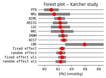
Both models demonstrate a high degree of consistency, with the random-effects estimate falling well within the fixed-effect confidence interval. Notably, these results are directly interpretable on the original measurement scale, nmol/kg for lead, without requiring back-transformation, simplifying the interpretation compared to log odds ratios in proportion-based meta-analyses, as shown in @fig-forest-lab. Note that we don’t need to draw a vertical line because we are not testing a specific null value.

#| label: fig-forest-lab
#| fig-cap: "Forest plot of Lead (Pb) concentrations from Karcher et al."

fig = res_karcher.plot_forest(
    use_exp=False,  # Linear scale is only required
)
fig.set_figwidth(3.5)
fig.set_figheight(3)

plt.title('Forest plot -- Karcher study')
plt.xlabel('[Pb] (nmol/kg)');

# Calculate the weighted effects by multiplying each effect by its fixed-effects weight
karcher_weighted = mean_karcher * res_karcher.weights_fe
#karcher_weighted = res_karcher.effect * res_karcher.weights_fe

# Calculate the pooled fixed effect by summing the weighted effects and 
# dividing by the sum of the weights
E_karcher_fe = karcher_weighted.sum() / res_karcher.weights_fe.sum()

# Calculate inverse variances and standard error (fixed-effect)
inverse_variance_karcher = 1 / std_karcher**2
SE_karcher_fe = 1 / np.sqrt(inverse_variance_karcher.sum())

# Calculate confidence interval (fixed-effect)
# If t-distribution is preferred, with k the number of studies
#t_crit_karcher = stats.t(df=res_karcher.df).ppf((1+.95)/2)
ci_lo_E_karcher_fe = E_karcher_fe - z_crit * SE_karcher_fe
ci_up_E_karcher_fe = E_karcher_fe + z_crit * SE_karcher_fe

print(f"Combined effect size in Karcher study (FE) = {E_karcher_fe:.5f}")
print(f"  with SE = {SE_karcher_fe:.4f}")
print(f"  and the 95% CI ranging from {ci_lo_E_karcher_fe:.4f} \
to {ci_up_E_karcher_fe:.4f}")

Combined effect size in Karcher study (FE) = 62.58340
  with SE = 0.1078
  and the 95% CI ranging from 62.3720 to 62.7948

print("Cochrane heterogeneity assessment in Karcher study:")
res_karcher.test_homogeneity()

Cochrane heterogeneity assessment in Karcher study:

<class 'statsmodels.stats.base.HolderTuple'>
statistic = 24.80189774185419
pvalue = 0.001679351463714887
df = 8
distr = 'chi2'
tuple = (24.80189774185419, 0.001679351463714887)

print(f"I² in Karcher study = {res_karcher.i2 * 100:.2f}%")

I² in Karcher study = 67.74%

# Print τ²
tau2_karcher = res_karcher.tau2
print("τ² (Karcher study) = ", round(tau2_karcher, 4))

# Calculate normalized random-effect weights
normalized_re_weights_karcher = res_karcher.weights_re / res_karcher.weights_re.sum()
print("Normalized random-effect weights:\n", normalized_re_weights_karcher.round(3))

τ² (Karcher study) =  0.288
Normalized random-effect weights:
 [0.123 0.04  0.16  0.123 0.09  0.071 0.17  0.194 0.029]

# Calculate combined effect size (random-effect)
E_karcher_re = (mean_karcher * normalized_re_weights_karcher).sum()

# Calculate inverse variances and standard error (random-effect)
re_weights_karcher = 1 / (std_karcher**2 + tau2_karcher)
#re_weights_karcher = res_karcher.weights_re
SE_karcher_re = 1 / np.sqrt(re_weights_karcher.sum())

# Calculate confidence interval (random-effect)
ci_lo_E_karcher_re = E_karcher_re - z_crit * SE_karcher_re
ci_up_E_karcher_re = E_karcher_re + z_crit * SE_karcher_re

print(f"Combined effect size (RE) = {E_karcher_re:.3f}")
print(f"  with SE = {SE_karcher_re:.4f}")
print(f"  and the 95% CI ranging from {ci_lo_E_karcher_re:.4f} \
to {ci_up_E_karcher_re:.4f}")

Combined effect size (RE) = 62.390
  with SE = 0.2457
  and the 95% CI ranging from 61.9085 to 62.8718

Standardized mean difference (SMD)#

Effect sizes like mean differences or standardized mean differences (SMDs) are employed to summarize the treatment impact. It is a statistical measure used to combine the results of studies that have measured the same outcome using different scales. It quantifies the difference between the means of two groups (e.g., treatment and control) divided by the standard deviation, effectively expressing the treatment effect in standard deviation units.

This allows for the comparison of studies that used different measurement tools, making it particularly useful when synthesizing continuous data where direct mean differences are not comparable. Common variations include Cohen’s d and Hedges’ g, which adjust for small sample bias, providing a standardized way to assess the magnitude of an effect across diverse studies.

The following example is based on the code from the statsmodels meta-analysis tutorial, with minor cosmetic changes applied for clarity and presentation.

# Define the row names (study identifiers)
study_smd = np.array(['Carroll', 'Grant', 'Peck', 'Donat', 'Stewart', 'Young'])
# Define the array of mean values of the treatment group
mean_t_smd = np.array([94, 98, 98, 94, 98, 96])
# Define the array of standard deviation values of the treatment group
sd_t_smd = np.array([22, 21, 28, 19, 21, 21])
# Define the array of number of observation in the treatment group
n_t_smd = np.array([60, 65, 40, 200, 50, 85])

# Define the arrays for the control group
mean_c_smd = np.array([92, 92, 88, 82, 88, 92])
sd_c_smd = np.array([20, 22, 26, 17, 22, 22])
n_c_smd = np.array([60, 65, 40, 200, 45, 85])

To calculate standardized mean differences, we use the effectsize_smd function. This function computes the effect size as the difference between the means of two groups (mean1 - mean2) standardized by an estimate of the within-group variance.

By standardizing the mean difference, we account for variations in measurement scales across the two groups, enabling us to compare studies that use different units of measurement for the same underlying construct.

Importantly, this function also allows for bias correction, such as Hedges’ g, which adjusts for small sample bias, ensuring more accurate effect size estimation, particularly when sample sizes are limited.

from statsmodels.stats.meta_analysis import effectsize_smd

# Computing bias corrected estimate of standardized mean difference
# and estimate of variance of smd_bc
smd_bc, var_smbd = effectsize_smd(
    mean1=mean_t_smd,
    sd1=sd_t_smd,
    nobs1=n_t_smd,
    mean2=mean_c_smd,
    sd2=sd_c_smd,
    nobs2=n_c_smd)

We then combine these standardized mean differences using meta-analysis techniques utilized throughout the chapter, to estimate the overall effect size across all studies, and generate the corresponding forest plot (@fig-forest-smd).

res_smb = combine_effects(
    effect=smd_bc,
    variance=var_smbd,
    method_re="dl",  # Same as 'chi2'
    use_t=False,
    row_names=study_smd)

# Print formatted summary results
print("\nMeta-analysis summary (SMD):\n", res_smb.summary_frame().round(4))

Meta-analysis summary (SMD):
                       eff  sd_eff  ci_low  ci_upp    w_fe    w_re
Carroll            0.0945  0.1827 -0.2635  0.4526  0.1239  0.1575
Grant              0.2774  0.1763 -0.0681  0.6229  0.1330  0.1628
Peck               0.3665  0.2256 -0.0756  0.8087  0.0813  0.1262
Donat              0.6644  0.1027  0.4630  0.8658  0.3916  0.2327
Stewart            0.4618  0.2083  0.0535  0.8701  0.0953  0.1379
Young              0.1852  0.1537 -0.1161  0.4865  0.1749  0.1827
fixed effect       0.4150  0.0643  0.2889  0.5410  1.0000     NaN
random effect      0.3585  0.1055  0.1518  0.5652     NaN  1.0000
fixed effect wls   0.4150  0.0992  0.2205  0.6095  1.0000     NaN
random effect wls  0.3585  0.0903  0.1814  0.5355     NaN  1.0000

#| label: fig-forest-smd
#| fig-cap: "Forest plot of Hedges' g standardized mean difference from the SMD example"

fig = res_smb.plot_forest(
    use_exp=False,  # Linear scale is only required
)
fig.set_figwidth(3.5)
fig.set_figheight(3)

plt.title('Forest plot -- SMD example')
plt.xlabel("Hedges' g");

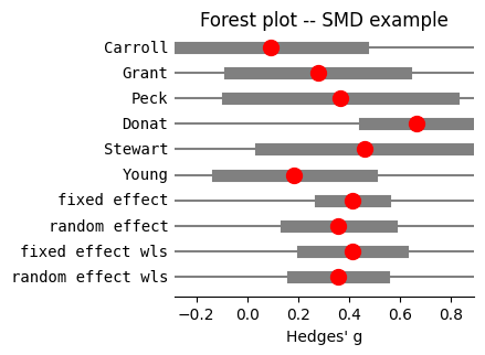
Hedges’ g is a refinement of Cohen’s d, we encounterd in @sec-statistical-power-and-sample-size, @sec-comparing-two-unpaired-means, @sec-comparing-paired-data, and @sec-comparing-models, specifically designed to address bias in small samples. Both measures are critical for power analysis and provide valuable information alongside t-test results. As we discussed earlier, a precise estimation of the effect size is important for the power of a study.

Meta-analysis of counted data#

# Calculate effect sizes (log odds ratios) and variances
eff, var = effectsize_2proportions(
    count1=count1,  # count positive in treatment group
    nobs1=nobs1,    # number of observation in treatment group
    count2=count2,  # count positive in control group
    nobs2=nobs2,    # number of observation in control group
    statistic="odds-ratio")

# Perform fixed- and random-effects meta-analysis (chi2/DL method)
res = combine_effects(
    effect=eff,
    variance=var,
    method_re="chi2",  # One-step chi2/DL estimate for RE variance τ²
    use_t=False,
    row_names=row_names)

# Print the summary results
res.summary_frame()          # LogOR
np.exp(res.summary_frame())  # OR

# Retrieving key information
res.effect
res.mean_effect_fe
res.weights_fe
res.df  # Degrees of freedom
res.mean_effect_re
res.method_re
res_eyding.tau2
res.weights_re

Mantel-Hanszel odds-raio#

import statsmodels.stats.api as smstats

# Construct the 2 x 2 x k contingency table, containing
# event and non-event counts, in treatment and control
counts = np.column_stack(
    [count1, nobs1 - count1, count2, nobs2 - count2])
ctables = counts.T.reshape(2, 2, -1)

# Create a StratifiedTable object from the contingency table
# The contingency table is cast to float64 to ensure compatibility
st = smstats.StratifiedTable(ctables.astype(np.float64))

st.logodds_pooled           # Pooled log odds ratio
st.logodds_pooled_se        # Standard error of the pooled logOR
st.logodds_pooled_confint() # Confidence interval of the pooled logOR

# Test of the null hypothesis that the pooled LogOR is 0 (OR=1)
st.test_null_odds()

# MH summary table
st.summary()

Heterogeneity#

# Cochran's Q χ² test
res.test_homogeneity()

# I²
res.i2

Meta-analysis using the t-distribution#

res = combine_effects(
    effect=eff,
    variance=var,
    method_re="chi2", 
    use_t=True,
    row_names=row_names)

res.conf_int_samples(
    nobs=np.array(data['nobs1'] + data['nobs2']))

Forest plot#

res.plot_forest(
    use_exp=True, # to show OR instead of logOR
)
plt.axvline(x=1, ls='--', color='blue')
plt.xscale('log')

Meta-analysis of continuous data#

# Overall effect size and variance
res = combine_effects(
    effect=mean,
    variance=std**2,  # variance
    method_re="dl",
    use_t=False,
    row_names=rownames)

# Computing bias corrected estimate of SMD and variance
smd_bc, var_smbd = effectsize_smd(
    mean1=mean1,  # mean values in group A
    sd1=sd1,      # standard deviation in group A
    nobs1=n1,     # total count in group A
    mean2=mean2,  # mean values in group B
    sd2=sd2,      # standard deviation in group B
    nobs2=n2      # total count in group A
)